Methods
Data Collection
By using a general rejection sampling approach and using the flexibility of the pan-tilt joints of the robots neck we were able to collect a large dataset of different robot configurations quickly.
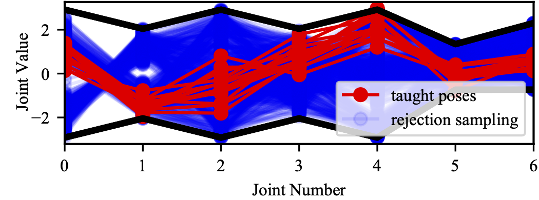 The different distributions in configuration space of the right arm with seven joints.
In red are the taught poses and our configurations resulting from the rejection sampling approach in blue.
The joint limits are in black.
The different distributions in configuration space of the right arm with seven joints.
In red are the taught poses and our configurations resulting from the rejection sampling approach in blue.
The joint limits are in black.
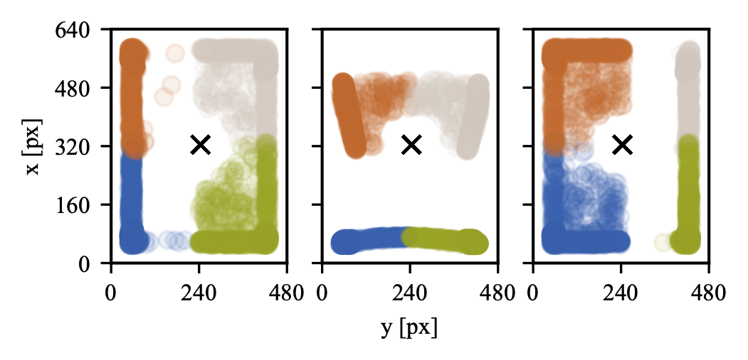 The different marker positions in the image for the left arm, the pole on the floor and the right arm.
We move the pan-tilt joints of the robot’s neck to get a good coverage of the image over all markers.
The different marker positions in the image for the left arm, the pole on the floor and the right arm.
We move the pan-tilt joints of the robot’s neck to get a good coverage of the image over all markers.
Virtual Noise
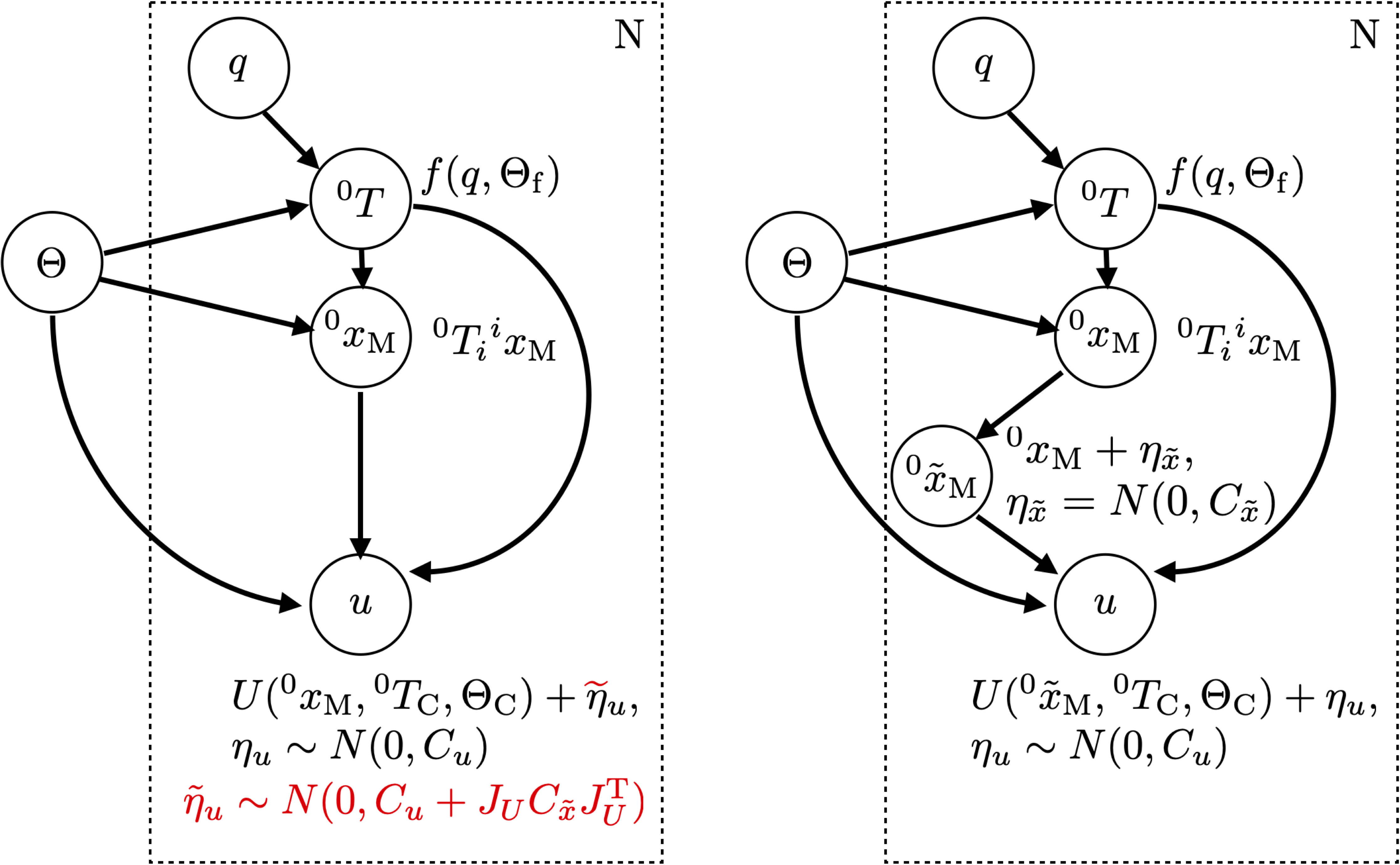 Probabilistic graphical model of the calibration problem including the camera and robot model.
For each of the \(N\) samples, it describes how the pixel coordinates \(u\) of a marker is computed from the joint configuration \(q\) and the model parameters \(\Theta\).
Left (w/o red parts): Original mapping with the real pixel measurement noise \(\eta_u\) as the only source of stochasticity.
Right: An additional virtual cartesian noise node is added to compensate for the imperfect (actually deterministic) kinematic model.
Left (with red parts): The virtual noise can be incorporated into the original model, resulting in an effective pixel noise with a \(\tilde{\sigma}_u\) depending on the distance of the marker to the camera (\(\propto 1/z^2\)).
Probabilistic graphical model of the calibration problem including the camera and robot model.
For each of the \(N\) samples, it describes how the pixel coordinates \(u\) of a marker is computed from the joint configuration \(q\) and the model parameters \(\Theta\).
Left (w/o red parts): Original mapping with the real pixel measurement noise \(\eta_u\) as the only source of stochasticity.
Right: An additional virtual cartesian noise node is added to compensate for the imperfect (actually deterministic) kinematic model.
Left (with red parts): The virtual noise can be incorporated into the original model, resulting in an effective pixel noise with a \(\tilde{\sigma}_u\) depending on the distance of the marker to the camera (\(\propto 1/z^2\)).